This tutorial provides
an overview of using BNW to build a Bayesian network model from a dataset and use the network to make predictions. The dataset used in this tutorial is a synthetic example of a genetic dataset that has a total of 8 variables. Two of the variables are genotypes labeled Geno1 and Geno2, and the remaining 6 variables are gene expression levels or other quantitative traits that are labeled Trait1 to Trait6. The dataset is available here.
The data file is formatted according to the guidelines on the BNW help page. The first row of the file contains the names of the variables and the remaining rows contain the data for each sample of the dataset. The genotypes (Geno1 and Geno2), which have two possible states (1 and 2), are the only discrete variables in the network. The quantitative traits are continuous variables.
1. Structure learning using default options
We do not know the network structure that underlies the relationships between the variables in this dataset, so we will use BNW to learn the structure that best explains the data. To begin, select Learn a network model from data from the BNW home page. Next, click Choose File at the top of the file upload page, navigate to and select the data file, and click Upload. A screen similar to image shown below should be displayed.
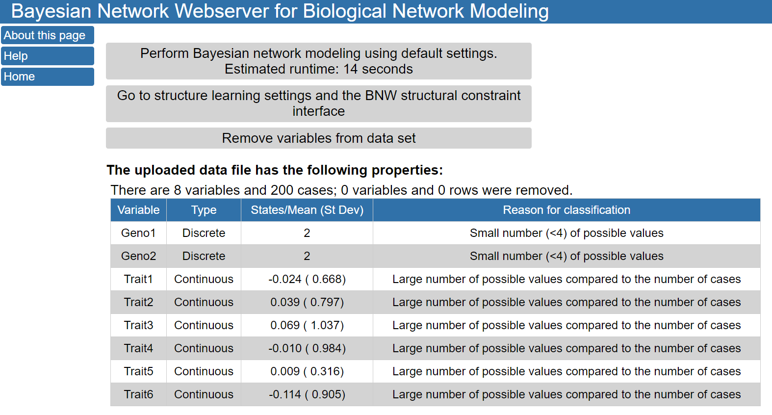
The buttons on the top of the page allow you to perform Bayesian network modeling using default settings; modify structure learning settings and add structural constraints; or remove variables from the data set. Under these buttons, a description of the loaded data set is provided, including if BNW classified the variables as discrete or continuous. In this case, the uploaded data file contained 8 variables and had 200 cases. Two variables (Geno1 and Geno2) were determined to be discrete variables because they had only 2 different values in the input data file. The other six variables were continuous variables with the means and standard deviations shown in the table.
2. Modifying structure learning settings In order to test if edges present the single best scoring network are conserved across high scoring networks, we can modify the structure learning settings to identify the structures of many high scoring networks and perform model averaging over these structures. To do this, click the Modify network strucutre button on the left of the page, opening a menu with three options that can be used to modify the network structure. Add or remove edges from network provides an interface for making specific changes to the network structure. The use of this interface is discussed here. In this tutorial, we are examining the impact of changing the settings used during structure learning on the network structure and click on Modify structure learning settings. We then select Go to structure learning settings and the BNW structural constraint interface on the resulting page. A more detailed overview of use of the structural constraint interface is provided in another tutorial.
3. Using the network structure to make predictions The network model can be used by make predictions through an interactive interface after clicking on the Use network to make predictions button on the left menu. To make predictions with the network, we will use the structure learned after model averaging of the top 1000 highest scoring networks. First, we will use the model to compare the expected values for nodes in the network based on observed genotypes. For these predictions, we will use evidence mode when making predictions, which is the default behavior in BNW. The difference between evidence and intervention modes is discussed in the BNW FAQ page. To use the model to make predictions based on Geno1, click on one of the blue bars in the Geno1 node and enter 1 or 2 to indicate which genotype value should be used to predict the values of the other network nodes. In the figure below, Geno1 is outlined in red and state 2 has a 100% probability, indicating that the value of this node has been entered as evidence. The red lines in the figure show the predicted distributions of the nodes after this evidence is known and can be compared with the blue lines which show the distributions for variables using the original data.
Initially, we will perform structure learning using default options in BNW and click on the Perform Bayesian network modeling using default settings button. By default, BNW limits the maximum number of parents for any node in the network to 4 and presents the structure of the single highest scoring network. Structure learning can take a significant amount of time for larger networks. For this dataset, structure learning should take only a few seconds, and the structure below will soon be displayed. The network can be also be accessed here.
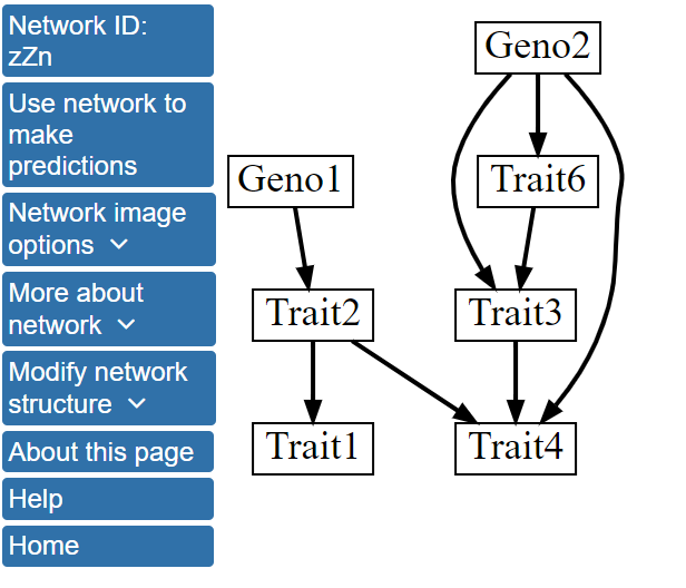
In the single best scoring network structure, the genotype nodes, Geno1 and Geno2, directly influence Trait2 and Traits3, 4, and 6, respectively. There are also several direct interactions between traits; for example, Trait2 influences Trait1 and Trait4. Additionally, Trait5 is absent from the network, indicating that this variable did not interact with the other variables strongly enough to be located within the highest scoring network.
Here, we only change the Number of networks to include in model averaging to 1000 and select Continue to assign variables to tiers. In this case, we will not assign variables to tiers, and can immediately click Click here to perform Bayesian network modeling after creating tiers. Now, instead of displaying the single highest scoring network, BNW will determine the 1000 highest scoring networks, perform model averaing over these networks, and display the structure after model averaging that includes all features with a Model averaging edge selection threshold greater than 0.5. Model averaging over the 1000 highest scoring structures has resulted in a change in the network structure as shown below and is available here.
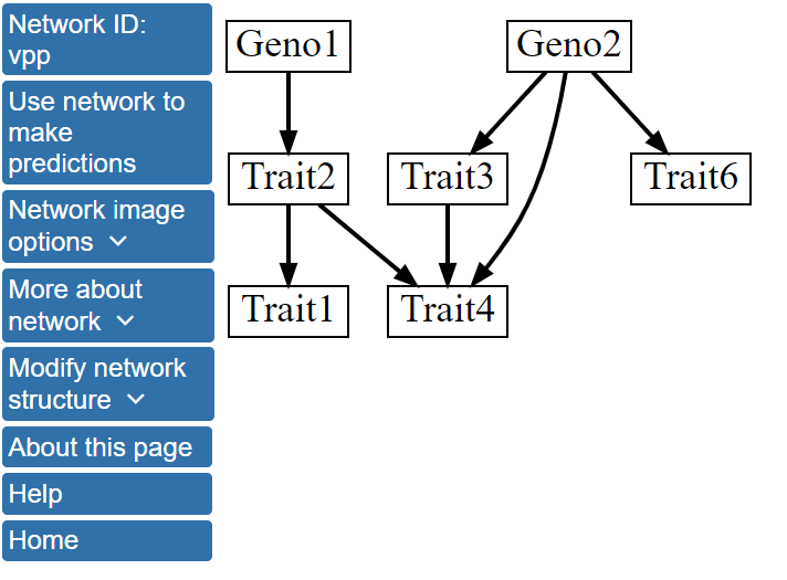
Specifically, the single best model network contains a directed edge linking Trait6 with Trait3, while this edge is absent from the structure after model averaging over the 1000 best scoring networks. More information about the network structure can be viewed by clicking Network image options on the left menu and, then, Show network with edge weights. The network structure with the edges labeled by their scores after model averaging will be displayed.
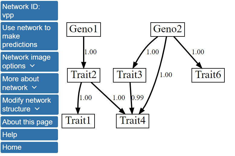
The model averaging scores show that the edges in this network model were found in all or nearly all of the 1000 highest scoring networks, and, thus, have scores of 0.99 or 1.00. For example, edges from Geno2 to Traits 3 and 4 have scores of 1. The model averaging scores for all possible directed edges in the network can be found by clicking View structure matrix under the More about network menu. The data provided in the structure matrix shows that the edge from Trait6 to Trait3 that was observed in the single highest scoring network has a posterior probability of 0.40, and it, therefore, falls short of being included in the model averaged network structure. The structure matrix file can be downloaded and used in return sessions to BNW, allowing users to skip structure learning and more quickly use the model to make predictions.
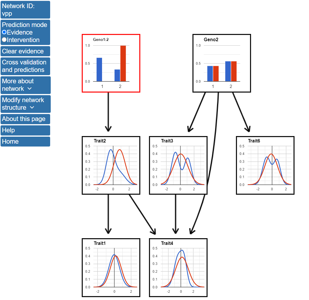
If Geno1 has genotype 2, the value of Traits 1, 2, and 4 are expected to increase compared with the distribution for all data. Specifically, the mean value of Trait2 is expected to be near 1 for Geno1=2 data, while it is close to 0 when this evidence is not known. Traits 1 and 4 are also expected to increase, but the magnitude of this increase is not expected to be as large.
To quantitatively assess the impact of this evidence on the network predictions, the View parameters button within the More about network parameters and structure menu can be selected. Clicking this button brings up a pop-up window with the network parameters (i.e., the probability distributions of the states of discrete nodes and the means and standard deviations of the Gaussian distributions for continuous nodes) for both the original data set and the data when considering the entered evidence.
Evidence for multiple nodes can be considered at the same time by clicking on a new node in the network and entering a value. Alternatively, users can select Clear evidence to reset the network to show the orignial distributions in a new tab.
Next, we will make predictions using the intervention mode. To use the prediction mode, click the button next to Intervention at the top of the page. The Selected mode tab on the left of the screan should now display Intervention. The effects of experimental intervention on Trait2 can be predicted by clicking on the blue line in the Trait2 node and entering a value for the variable. The figure below shows the network after setting Trait2 to a value of 1.5.
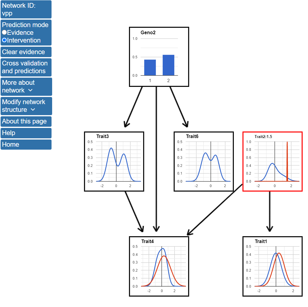
Entering a value for Trait2 in intervention mode results in a change in the structure of the network. Specifically, as Trait2 is now set by the experimental intervention, it is no longer dependent on its parents. In this case, as Geno1 was only connected to the network by being the parent of Trait2, Geno1 no longer appears in the network. Also, intervention mode only predicts how nodes that are descendants of Trait2 are affected. Setting Trait2 to 1.5 results in increases in the predicted values of both Trait1 and Trait4.